Two-Stage PON Splitting: Design Guide

Most two-stage PON designs are inherited, not designed. A planner takes the 1:32 the network was costed around, notices the distribution cable is 32 fibres wide and expensive to pull, moves a 1:8 splitter out to the access terminal, and calls it a 1:4 plus 1:8. The ratio is unchanged, the fibre count drops by three quarters, and the design goes out the door.

Then the first ONT on the last branch fails to range, or it ranges today and stops ranging in year four when a splice case fills with water, and the question becomes why nobody added up the decibels on the worst path instead of the average one.

Two-stage splitting is not a re-arrangement of a ratio. It is a decision about where the light divides, and every consequence — loss, port utilisation, fault isolation, test access, the upgrade path — follows from that placement. This guide treats two-stage PON splitting in the order an engineer has to defend it: what the second stage costs optically, how the worst path is budgeted, how each stage is sized, and where the hardware goes.

If you have not settled the overall ratio yet, start with splitter ratio selection and come back — this article assumes the total ratio is decided and the open question is how to build it. The FTTH and PON deployment guides cover the wider architecture picture.

Two-stage splitting is a placement decision, not a ratio

A splitter ratio counts output ports. A split level counts how many devices the light passes through. A 1:32 can be one module in a cabinet or a 1:4 in a street closure feeding four 1:8s in access terminals — identical ratio, identical subscriber count, different optical budget, different fibre count, different operational life. Call it two stage PON splitting or a cascaded split architecture — the label changes nothing about the decibels, only where they are spent. A two-level splitter of 1:4 then 1:8 reaches the same 32 ports through two devices and one more patch point.

The Fiber Broadband Association's splitter architecture primer draws the distinction cleanly: a provider fixes an overall ratio, then uses "2 or more splitter combinations to arrive at the target split ratio," with 1:4 plus 1:8 making a 1:32 and 1:2 plus 1:16 another common pair. Cascading is the mechanism; the design work is choosing the decomposition.

That decomposition is where the money and the risk sit, because the two stages answer two different questions:

• Stage one is a geography question. How many separate places do I need to reach with my own fibre? Its ratio equals the number of second-stage sites you can feed from one OLT port.
• Stage two is a density question. How many premises sit inside each of those places? Its ratio equals homes passed per terminal.

Get those backwards — size stage one by subscriber count, stage two by street count — and the network strands capacity at one end while running out of reach at the other.

What the second stage actually costs on the optical path

Every splitter stage adds insertion loss, and a cascaded PON splitter does not make the arithmetic cheaper: two stages whose ratios multiply to 32 cost slightly more than one 1:32 module, not the same.

The ideal split is the same either way: 10 × log₁₀(N), so 15.0 dB for 1:32 however you build it. The difference is excess loss, which grows with port count on a single device but is paid twice on two smaller ones. Commercial PLC modules usually quote worst-case insertion loss and worst-case uniformity; a representative 1×N datasheet gives 7.0 dB for 1:4, 10.2 dB for 1:8, 13.5 dB for 1:16 and 20.5 dB for 1:64, with uniformity of 0.6 dB at 1:4 and 0.8 dB at 1:8 (PLC splitter specification).

The figures in the table are the numbers the datasheet tabulates, which it does not label max or typ; treat them as worst-port figures. The table quotes insertion loss and loss uniformity as separate parameters: uniformity is the spread between the best and the worst output port, not an extra loss to add on top. Budget the insertion-loss figure and leave uniformity alone — unless your vendor quotes a typical figure for one port, in which case add the uniformity value to reach the worst port.

Run the decomposition through that table: the 1x4 and 1x8 splitter modules together carry 17.2 dB of insertion loss against 16.5 dB for a single 1:32 — 0.7 dB more for the same 32 ports, and that is the whole of the PON splitter cascade loss on paper. The Fibre Optic Association's FTTH design reference rounds the same cascade to 7 dB plus 11 dB, an 18 dB splitter bill.

Two more line items belong to the second stage specifically, and they are the ones budgets forget:

• An extra mated pair at the input unless the second stage is spliced in. Design practice allows 0.3 dB per mated pair for field-terminated SC/APC connections, and that is the figure this budget uses. Datasheets sometimes quote a different quantity — Fiberdyne's PS 4036 datasheet, for one, notes that its tabulated 1xN figures are “specified without connectors” and that you add 0.2 dB per connector when they are fitted: a per-connector adder, not a pair loss. If your assembly datasheet states a pair figure, compare it with the 0.3 dB allowance and take the higher of the two on the worst path.
• An extra splice or two on the distribution fibres reaching that enclosure, at roughly 0.1 dB each.

Add those and the real penalty for the cascade is 1.1–1.2 dB — 0.7 dB from the splitter line, 0.3 dB for the extra pair, 0.1–0.2 dB for the extra splice — not the 0.7 dB the splitter table alone suggests. That is the price of the fibre saving, and it has to be visible in the budget before the design is approved — not discovered at commissioning. The splitting-loss walkthrough covers the per-stage numbers if you want the full derivation.

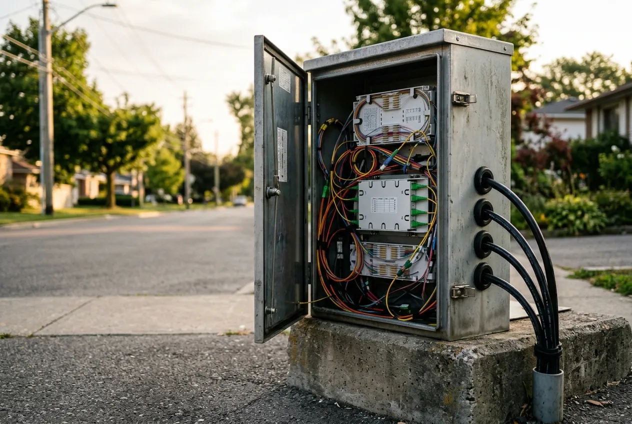
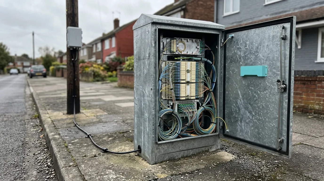
A first stage in a street cabinet: one feeder fibre in, four distribution cables out. The ratio is set by how many second-stage sites you can reach, not by how many homes you have.

The worst-path budget, worked end to end

Budgets fail on the longest, most-spliced, most-connectorised path in the ODN — never on the average. Here is a two-stage design costed that way.

Assumptions, all of which you should replace with your own route data: 9.2 km from the OLT to the furthest ONT (the ONU at the customer end), 10 fusion splices on that path, four mated connector pairs (OLT patch, cabinet patch, terminal input, ONT), 1:4 module in the cabinet, 1:8 module in the access terminal, fibre at 0.35 dB/km. The 0.35 dB/km figure is the value commonly quoted for G.652.D cable at 1310 nm; the G.652 recommendation defines the fibre class, and your cable datasheet gives the guaranteed number.

Against a GPON Class B+ budget of 28 dB (ITU-T G.984.2, the PMD layer that defines the optical path loss classes), that leaves 5.38 dB — above the 3 dB design margin most planning teams hold back for repairs, ageing and a future re-splice.

The same 32 ports built as a single 1:32 in the cabinet would need one mated pair fewer (no stage-two input) and one splice fewer (no second closure): 21.52 dB, leaving 6.48 dB. So the honest statement of the trade is: this cascade buys a four-fibre distribution cable at a cost of 1.1 dB of margin — 0.7 dB from the splitter line, 0.3 dB from the extra pair, 0.1 dB from the extra splice. If your route had 2 dB less headroom, this cascade would spend most of the reserve you keep for repairs — a harder call than the table alone suggests.

Two sensitivities worth running before you sign off:

• Add 3 km. Every kilometre costs 0.35 dB, so the cascade lands at 23.67 dB — still inside B+, margin down to 4.33 dB.
• Go to 1:64 as 1:4 plus 1:16. Splitter loss becomes 20.5 dB and the total 25.92 dB: 2.08 dB of margin, below the 3 dB reserve on Class B+. That design needs Class C+ (32 dB) or a shorter route. The class definitions are in G.984.2; do not assume a B+ network can absorb a 1:64 cascade without checking.

Sizing stage one: outputs equal second-stage sites

The most common sizing error is to pick stage one from the subscriber count. It should come from the map.

If a 1:4 sits in a street cabinet, it can serve four second-stage locations. If your serving area has nine terminal clusters inside affordable drop distance, a 1:4 leaves five of them unreachable from that cabinet, no matter how few subscribers they hold. The stage-one ratio is therefore bounded above by the number of second-stage sites you intend to build, and bounded below by the loss you can still afford.

Practical framing:

• One stage-one output per second-stage site, plus one spare where the duct route allows. A spare output on the cabinet is cheap; re-digging to add a fourth fibre is not.
• Stage one belongs close to the OLT. It exists to reduce fibre count on the longest, most expensive span. Pushing it far into the field saves almost nothing and costs the same decibels.
• A 1:2 or 1:4 at the OLT itself is a legitimate first stage when a single OLT port has to serve two or four widely separated areas — the ratio arithmetic still works, and it keeps the feeder count low.

The counter-argument is real and should be written down: every stage-one output that carries a part-loaded branch strands OLT port capacity, because the port is committed to 32 homes whether they subscribe or not. A 1:4 feeding four 1:8s in an area at 60% take serves around 19 subscribers from one OLT port. The cost comparison is per connected subscriber, not per port.

Sizing stage two: homes per terminal, take rate and stranded ports

Stage two sets the shape of the network's growth. The distributed split ratio at this level is homes passed per access terminal, and the number you actually care about is how many of those ports will still be dark in year five.

Two rules fall out of that table.

Match the module to the cluster, not to the catalogue tier. An 8-home cul-de-sac with a 1:16 terminal wastes half the module's outputs and its loss. A 16-home terrace with a 1:8 terminal cannot be served at all without a second fibre from the cabinet — the expensive failure, because the fix is civil work.

Reserve flexibility at stage two, not stage one. Swapping a 1:8 cassette for a 1:16 in an access terminal is a permitted module change; adding a fifth output to a 1:4 in a sealed cabinet is not. Where the local plan is uncertain, standardise on one module size for inventory simplicity and accept stranded capacity deliberately, in writing, rather than by accident.

One asymmetry is worth stating plainly, because it decides the whole architecture: a spare port in a centralised splitter can serve any home in the PON; a spare port in a cascade can only serve homes behind that branch. Cascading converts flexibility into fibre savings, and no amount of port arithmetic reverses that.

Where each splitter physically lives

Placement is not just "cabinet versus pole". Each location in the chain — central office or fiber distribution hub (FDH), street cabinet, splice closure, access terminal, in-building box — has a different failure mode, a different maintenance regime and a different cost of change.

The comparison of FAT and FDT access cabinets covers which enclosure suits which stage, and the FTTH topology design guide works through how the placement choice propagates into cable counts and route lengths.

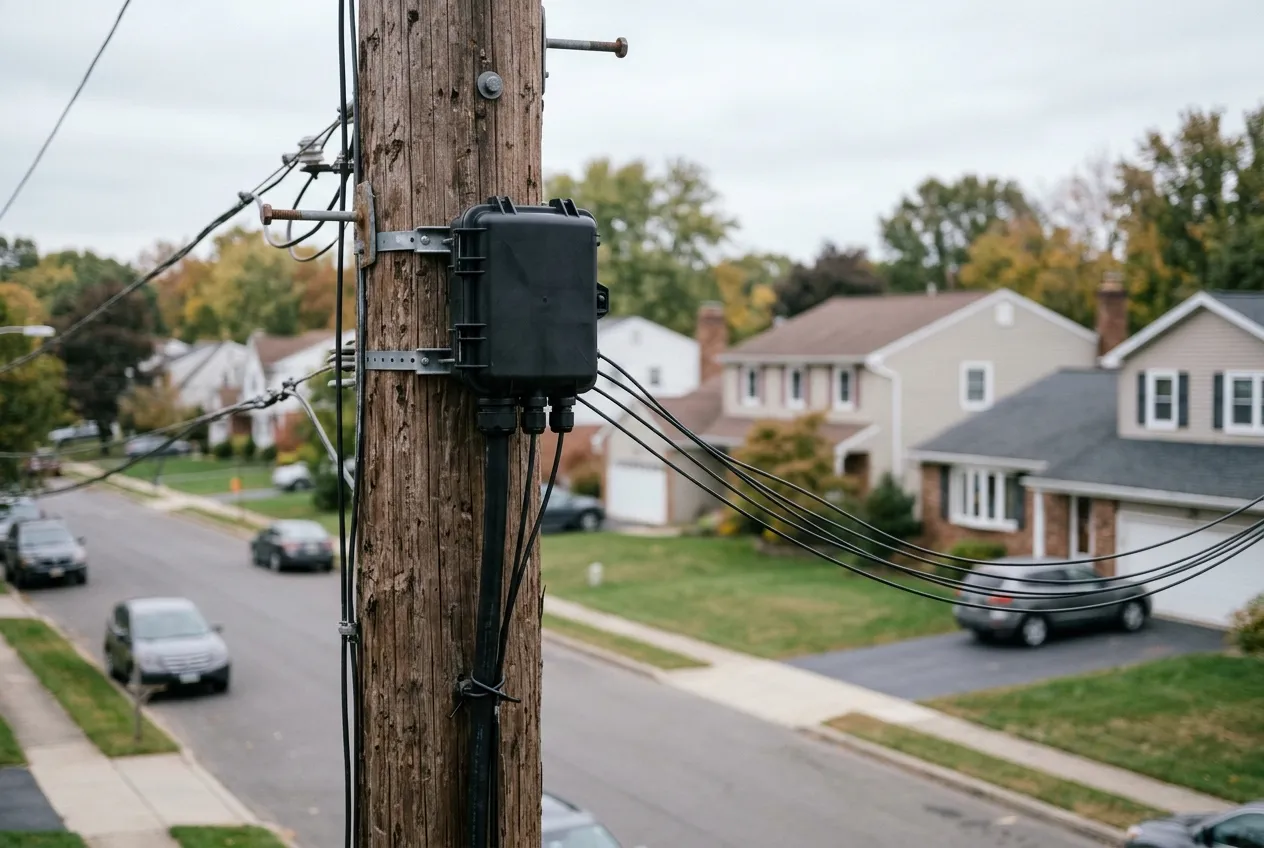
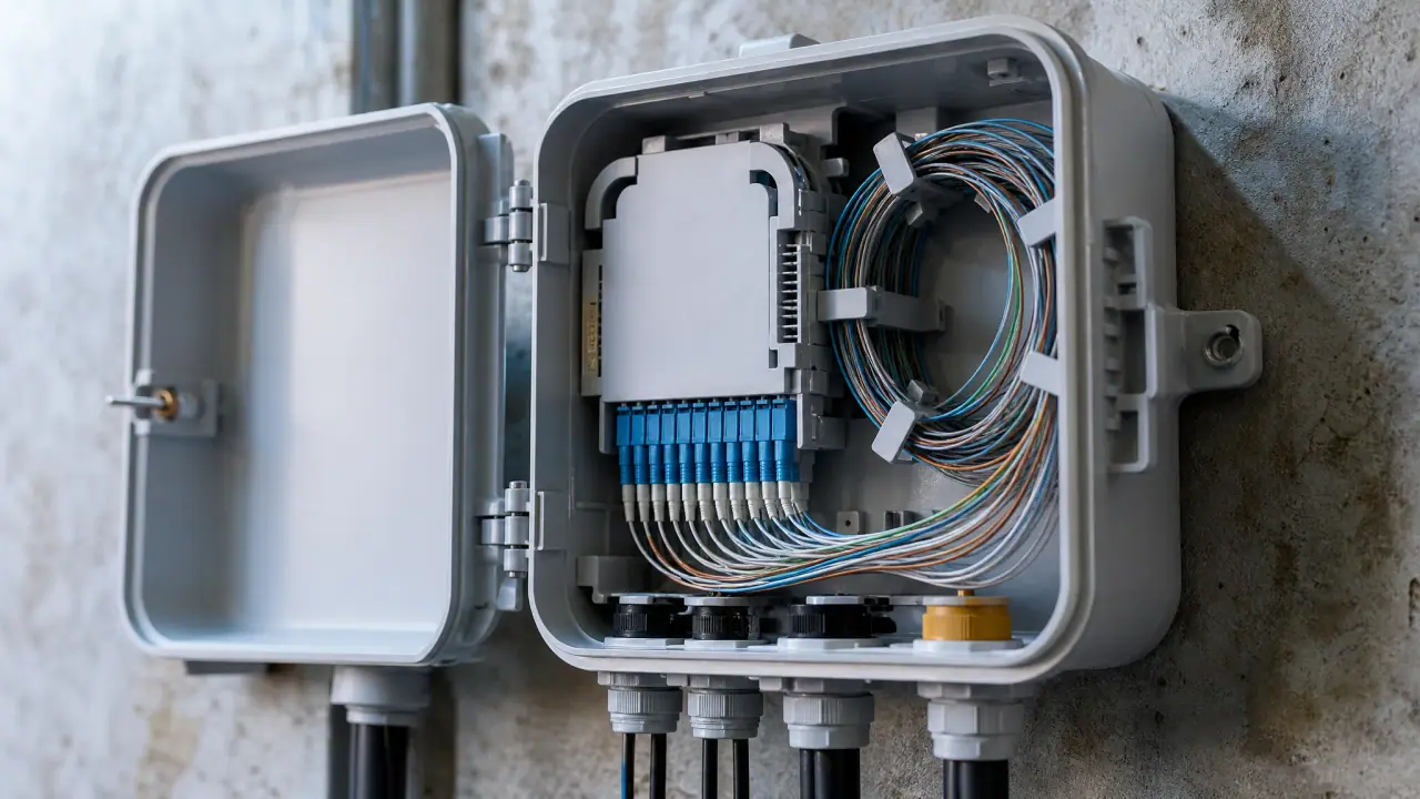
A second stage at the access terminal: the drops to the premises behind this terminal, served by one distribution fibre from the cabinet. This is where the cascade's fibre saving is actually realised.

Two placement constraints get ignored until they hurt:

• Spliced versus connectorised. Most cascaded builds are half-spliced, half-connectorised: feeder and distribution fibres spliced into the splitter, pre-connectorised adapters on the drop side. That choice determines whether a later module swap needs a splicer or a patch cord.
• Records. A two-stage network has one more passive node per branch to record than a single-stage one. If the splices are not documented in the same system as the ports, the first fault becomes an excavation.

The connectors and splices nobody budgets for

Budget discipline in cascaded designs fails in a predictable place: the small items around the second stage get counted once at design time and three times in reality.

Count them explicitly on the worst path:

1. OLT patch panel to OLT port — one mated pair.
2. Cabinet entry — a mated pair if the feeder is patched, a splice if it is not.
3. Stage-one input — splice or pigtail connector, depending on build style.
4. Stage-two input — the mated pair that a single-stage design does not have.
5. ONT — one mated pair, and an SC/APC adapter at the customer end.

At 0.3 dB per mated pair, the difference between a spliced cascade and a fully patched one is often 0.6–0.9 dB — the same order as the entire splitter penalty. A design that budgets "splitter loss plus a bit" will pass on paper and fail on the last house.

Splice allowances matter less per event but there are more of them: each closure in the cascade path contributes, and a two-stage design usually has one more closure than the single-stage equivalent.

What two stages do to testing and fault isolation

This is the part of the trade that never appears in a loss table.

An OTDR cannot see through a splitter with useful dynamic range — the return from beyond the splitter is buried, and with two stages the interpretation gets worse, not better. The Fibre Optic Association's GPON fault-finding manual is explicit that in a 1:4 plus 1:16 cascade, automated iOLM testing can only be performed from the ONT end, producing a customer-side view — which is why the manual insists the route profile must have the splitter stages defined correctly before any pass/fail analysis means anything.

The operational consequences:

• Test access moves to the customer. Every fault investigation starts at the premises, or at the terminal if you can isolate a branch. A single-stage design lets you test from the cabinet in both directions.
• Fault domain shrinks. A failed second-stage module takes out one branch — typically four to sixteen subscribers — instead of the whole 32. On a dense network that is a meaningful difference in SLA terms.
• Fault finding gets harder. Two stages mean two candidate splitter locations plus the distribution fibres between them, all of it invisible to a cabinet-side test.

If you plan to run proactive monitoring, budget for it at design time: reflective elements at the ONT, or a test head at the OLT with a high-dynamic-range solution. Neither is free, and retrofitting them to a sealed cascade is worse. The OTDR field guide covers trace interpretation and launch-cable practice.

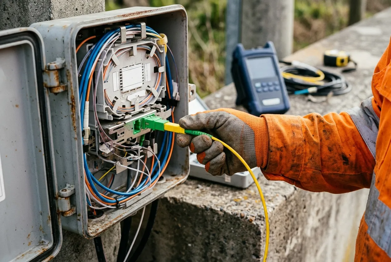
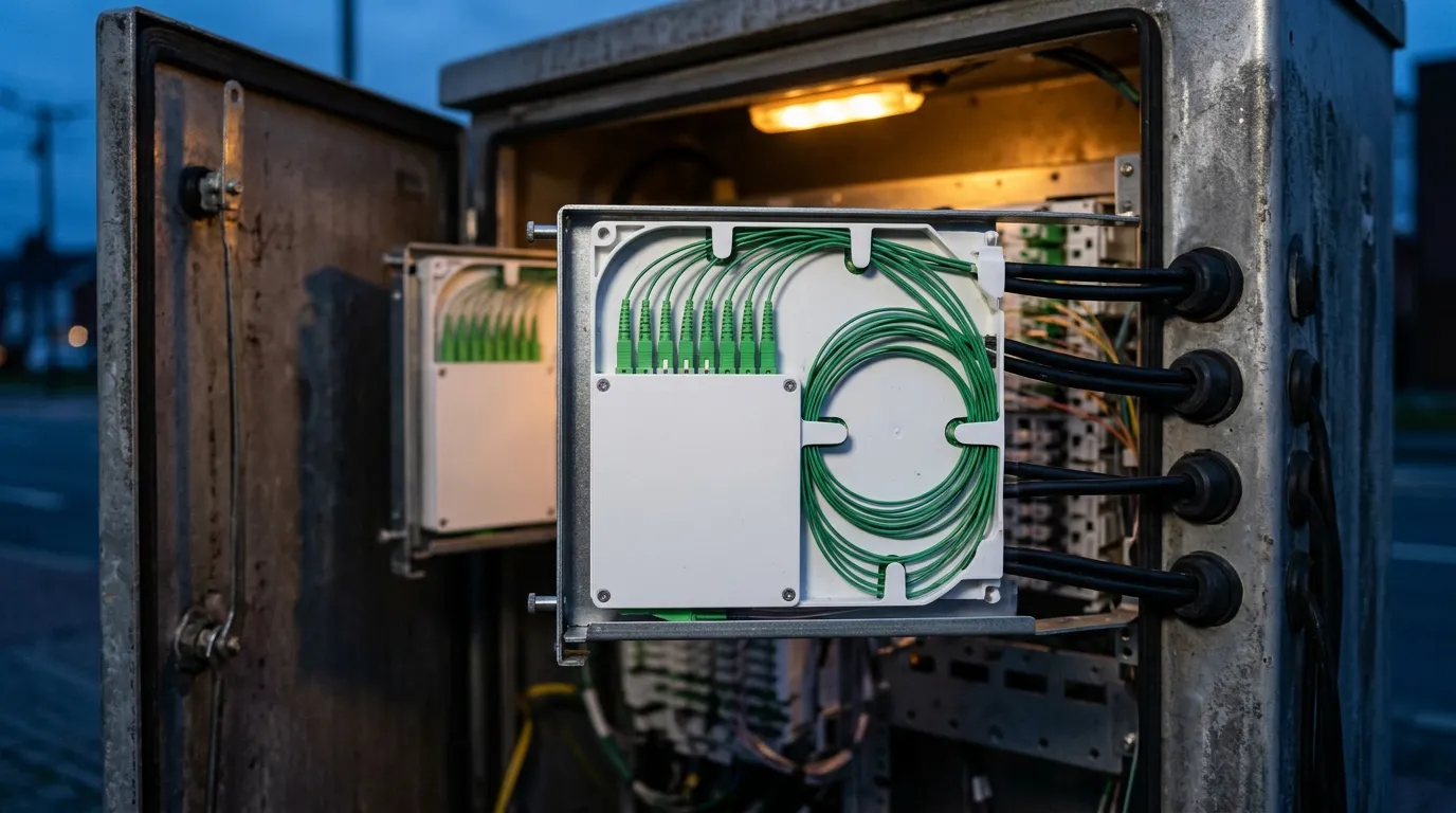
Test access in a cascade: the measurement starts at the customer end, because the splitter stages block a cabinet-side view of the drop.

Upgrading a cascade to XGS-PON

Two-stage networks built for GPON are usually expected to carry 10G later. Check that assumption with the numbers rather than the marketing.

XGS-PON path loss classes are defined in ITU-T G.987.2, with N1 allowing 29 dB. Against the worked example above (22.62 dB), that leaves 6.38 dB — comfortable. The failure case is a cascade originally built as 1:4 plus 1:16 for a 1:64: at 25.92 dB it clears N1 by only 3.08 dB, and on GPON it leaves 2.08 dB against Class B+ — under the 3 dB reserve before a single repair splice is made. That branch needs N2 (31 dB) or a shorter route.

Three rules that keep a cascade upgradeable:

• Keep at least 3 dB of margin on the GPON design even when the budget passes with less. That reserve is what buys the higher-loss optics class later.
• Do not consume the last spare stage-one output for a copper-era commercial reason. It is the only cheap way to add a second-stage site later.
• Power budget is not the only constraint. Higher split ratios also mean less bandwidth per subscriber at peak; a 1:64 cascade that passes optically can still be commercially wrong at 10G. The GPON / XG-PON / XGS-PON comparison covers the class and wavelength differences.

Note also that a cascade must be checked at the wavelengths it will actually carry: PON splitters are specified over 1260–1650 nm, and XGS-PON adds 1270 nm upstream, so a module qualified only at 1310/1550 needs its datasheet read, not assumed.

A design sequence you can hand to a reviewer

Run these in order; each one closes options for the next.

1. Fix the total ratio from the loss budget and the subscriber target — this is the ratio decision.
2. Map second-stage sites. Count the terminal clusters inside affordable drop distance. That count caps stage one.
3. Map homes per cluster. That sets stage two, per branch.
4. Decompose the ratio so the two stage ratios multiply to the target, and reject any decomposition that needs a module you do not stock.
5. Budget the worst path, element by element, with per-stage splitter maximums, every mated pair and every splice. Hold 3 dB.
6. Check the port economics at your realistic take rate: live subscribers per OLT port, dark ports per branch, cost per connected subscriber.
7. Choose enclosures and record the build style — spliced, connectorised, or mixed — for each node.
8. Write the test plan for a cascade, not a single-stage network: ONT-side iOLM, branch isolation procedure, documented splitter stages in the route profile.
9. Re-run the budget at N1 and at 1:64 so the upgrade answer is known before the first trench is opened.

A design that survives those nine steps can be defended in a review. One that skipped step 5 cannot, however elegant the topology drawing looks.

What TTI Fiber supplies for cascaded ODN builds

TTI Fiber manufactures the passive layer these designs are built from: PLC splitters from 1x2 to 1x64 in bare-fibre, ABS box, LGX module and rack-mount formats, with connectorised options, plus outdoor-rated drop cable and single-mode patch cords for cabinet and terminal patching. If you send us the stage decomposition you are working to and the worst path you need to clear, our engineering team will confirm which formats and connector options fit, and which module-level loss figures you should be budgeting against. If you would rather start from a module list, the PLC splitter module formats we build cover the 1x4 and 1x8 stages this design uses.