FAT vs FDT: Fiber Cabinets in FTTH Networks
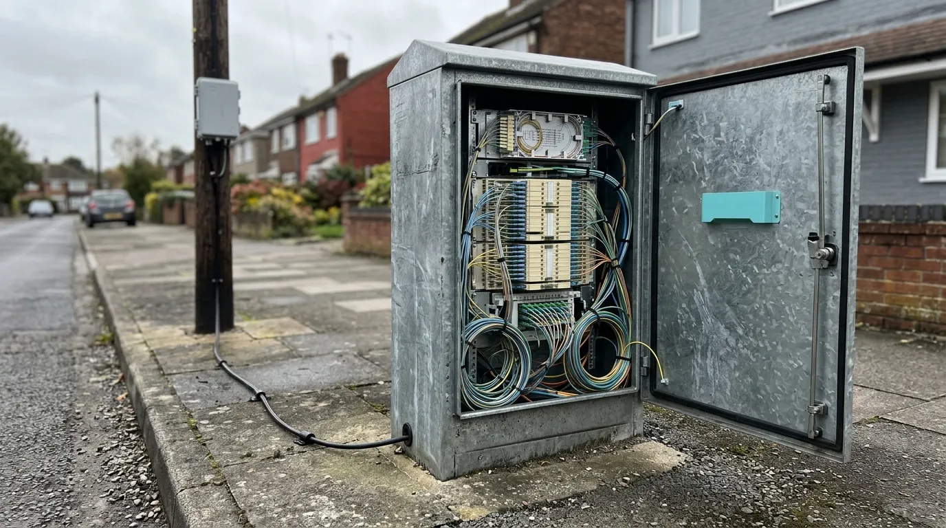
FAT vs FDT is not a choice between two interchangeable boxes — it is a question about which boundary each one sits on. In many FTTH architectures, the FDT or FDH is the node where feeder fibers are organized and may be spliced, cross-connected or split before distribution cables continue into the access network. The FAT is commonly the access-side terminal where distribution fibers are connected to subscriber drop cables, but the exact physical boundary and enclosure function depend on the operator’s architecture and vendor terminology. Put simply: the FDT changes how many cables you are dealing with, the FAT changes which house you are connecting. Everything else — port counts, enclosure ratings, splitter placement — follows from that split of duties. This guide is written for the people who have to specify and install both, and it sits inside the wider FTTH and PON deployment guides for last-mile access.
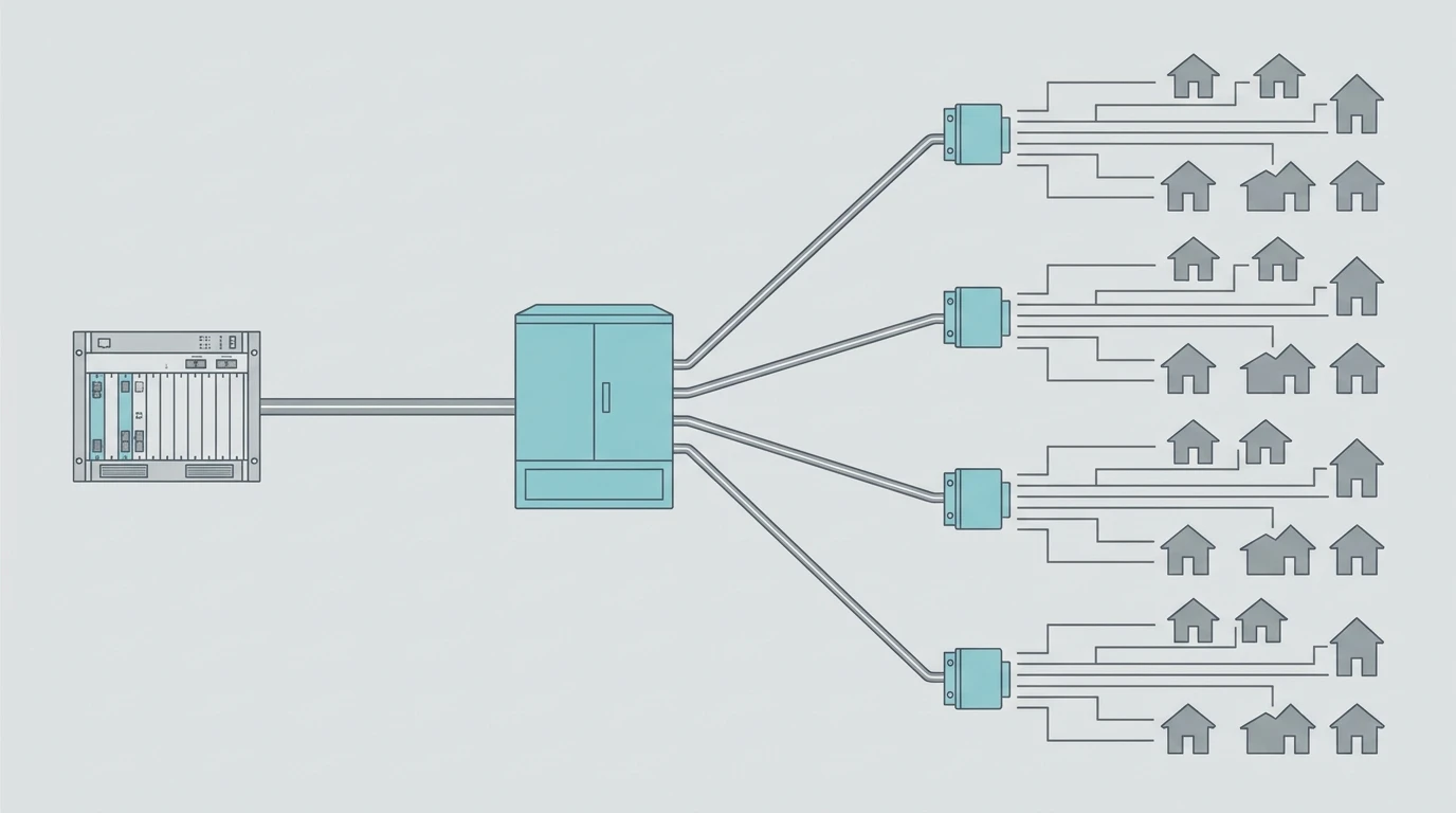
The boundary is the whole difference
In a PON, every enclosure sits on one of three fiber segments: the feeder from the OLT, the distribution cable through the streets, and the drop to the premises. Many PON designs use two main logical boundaries: feeder-to-distribution and distribution-to-drop. In practice, the physical functions may be split across an ODF, cabinet, splice closure, FDH, FAT or other terminal, depending on the operator’s architecture and vendor terminology.
FDT (fiber distribution terminal) / FDH (fiber distribution hub) | FAT (fiber access terminal) | |
|---|---|---|
Boundary it owns | Feeder → distribution | Distribution → drop |
What enters | One or more feeder cables, high fiber count | One or more distribution cables, typically with fewer fibers than the feeder cable |
What leaves | Many distribution cables | Individual drop cables |
Typical function | Splice, first-level split, cross-connect or patching | Splice, second-level split, drop adapters |
Ports | Representative planning ranges include 24–96 distribution ports and 12–48 feeder ports for some FDT/FDH designs | FATs commonly use 4-, 8- or 16-drop configurations. Actual counts depend on the operator’s architecture and the selected product |
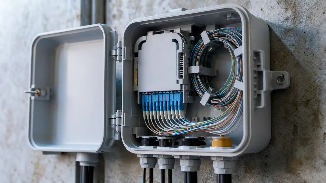
Enclosure | FDT/FDH products may be cabinet-, pedestal- or vault-mounted, while FAT products may be wall-, pole- or strand-mounted | Materials, door configuration and protection level depend on the installation environment and product design |
Splitter | Usually present (level 1) | Often present (level 2) |
Failure blast radius | Potentially many subscribers served through that node; the actual scope depends on the feeder, splitter, cross-connect and redundancy design | Typically the customers connected through that FAT; the actual scope depends on the port count and network architecture |
Directly terminates subscriber drops in a conventional architecture | Usually no | Usually yes |
The row that matters most is the last one. A technician standing at an FDT is working on a network; a technician standing at a FAT is working on a customer. That difference sets the enclosure, the access requirements, the IP rating and the way you record the plant — far more than the splitter inside either box.
Where the boundary sits inside a two-level split
The most common misunderstanding in this comparison is that the FDT/FAT distinction is about where the splitter lives. It is not. Splitter location is a design choice; the feeder/distribution and distribution/drop boundaries are physical facts. The three classic recipes — home run, centralized split and distributed split — use different combinations of ODFs, splice closures, FDTs and FATs. Centralized- and distributed-split designs commonly use FATs, while a home-run design may use another splice or termination point instead. Cabinet presence should not be inferred from splitter location alone.
A total split ratio of 1:32 can be built three ways, and only the third puts a splitter in both boxes:
- Single-level, splitter at the FDT. One 1:32 splitter at the cabinet, and every FAT becomes a passive splice-and-patch box. Clean and cheap in hardware, but each subscriber then needs a dedicated distribution fiber — 352 subscribers means 352 fibers leaving one cabinet. Rarely practical.
- Single-level, splitter at the FAT. One 1:32 splitter in each access box. Cheap on distribution fiber, but the weight and cable bundle of a 32-port box at a pole can be difficult to manage, and a single splitter fault takes 32 homes down.
- Two-level. 1:4 at the FDT and 1:8 at the FAT. This arrangement is common in many FTTH deployments, but the preferred architecture depends on operator practice, subscriber density, civil cost, optical budget and maintenance strategy. It is therefore an arrangement that especially requires explicit capacity and optical-budget sizing.
In the two-level case, the ratios are mathematically interchangeable only in total split, not in their impact on distribution-fiber count, FAT capacity, node count and optical topology. At a fixed total split, the first-level ratio decides how many distribution fibers you pull, and the second-level ratio decides how many drops each FAT carries:
Level 1 at FDT | Level 2 at FAT | Distribution fibers per OLT port | FATs needed for 384 drop ports | Drops per FAT |
|---|---|---|---|---|
1:2 | 1:16 | 2 | 24 | 16 |
1:4 | 1:8 | 4 | 48 | 8 |
1:8 | 1:4 | 8 | 96 | 4 |
All three rows deliver the same nominal 32-way split. Their ideal splitter losses are similar, but the actual cascade loss depends on the specified insertion loss, excess loss, uniformity, connector loss and splice count of each selected splitter assembly. What changes is the cost, and it moves in one direction only: heavier level-1 splitting multiplies both the distribution fiber count and the number of boxes on the street. Going from 1:2/1:16 to 1:8/1:4 takes distribution fibers from two per OLT port to eight and FATs from 24 to 96, because a four-drop box serves a quarter as many homes as a sixteen-drop box. What the extra boxes buy is small enclosures and a small outage footprint — four homes behind each door instead of sixteen. So heavy splitting at the FDT is the right call when distribution cable and duct are cheap to build, when the FAT positions are tight (a pole mounting or a narrow wall that will not take a sixteen-drop box), and when a single fault must not take sixteen homes down; the price is approximately four times as many FAT positions and distribution fibers in this 384-drop example, together with potentially more installation and maintenance visits. It is the wrong call when the goal is fewer boxes or fewer visits, and it does not automatically reduce truck rolls because each new connection may still require a FAT visit unless the operator uses pre-terminated drops, remote activation or another staged-connection process. Split lighter at the FDT (1:2/1:16) when distribution fiber and duct capacity are expensive and each enclosure can be large — 24 boxes, sixteen drops each, one door to open for sixteen customers.
The optical cost is real but modest. As representative planning values, a PLC 1:4 may contribute about 7.3 dB and a 1:8 about 10.7 dB, so a 1:4 + 1:8 cascade is near 18 dB, compared with roughly 17 dB for a single 1:32. The actual maximum loss must come from the selected splitter data sheets, including excess loss and connector configuration — plus the extra connector pairs at the second splitter. On a GPON Class B+ system, which is commonly associated with a 28 dB maximum optical-path-loss class, that may remain workable within the available design margin. However, the applicable OLT/ONT class, component losses, design margin and project acceptance criteria must still be verified. On a long-reach or high-split design, the splitter cascade should be modeled before the enclosures are ordered, which is why splitter ratio selection and the loss a passive splitter adds are worth settling before you order enclosures. XG-PON and XGS-PON can support higher split configurations, commonly up to 1:128 in deployed designs. The usable ratio is not an unconditional limit set by the recommendation alone; it depends on the OLT/ONT optical class, reach, splitter and connector losses, fiber topology, and the operator’s design rules. Verify the applicable ITU-T optical specifications and the selected equipment data sheets before adopting 1:128. The nominal split-loss arithmetic remains the same, but the usable design still depends on the selected optical class, wavelength-dependent component performance, connector and splice losses, reach and required design margin.
Sizing math: how many subscribers per cabinet
Port counts on a datasheet tell you what a box can hold. Sizing tells you what to buy. The inputs are homes passed, take rate at the end of the planning horizon, total split ratio, and a spare-port policy.
Worked example — one FDT service area:
- Homes passed: 640.
- Take rate at year 3: 55% → 352 subscribers.
- Total split: 1:32 as 1:4 at the FDT and 1:8 at the FAT.
- OLT ports: 352 ÷ 32 = 11 → provision 12 (one spare port).
- Feeder fibers: one per OLT port → a 12-fiber feeder cable.
- At year 3, 352 active subscribers require 44 occupied 8-drop positions; rounding to 48 FATs provides 384 drop ports for that deployment phase. If the outside plant must be physically ready for all 640 homes passed, size FAT locations, distribution fibers and drop capacity from the 640 premises plus the stated spare policy. At eight drop ports per FAT, the base count would be 80 FATs before adding spare capacity and adjusting for street geometry.
- Distribution fibers for the year-3 active phase: one per planned FAT position, so 48 positions require 48 fibers, or four 12-fiber elements. If the outside plant must be physically ready for all 640 homes passed, recalculate the final FAT count, distribution-fiber count and route topology for that full-build condition instead of retaining 48 as the complete-build count.
- Level-1 splitters for the year-3 active phase: 12 × 1:4, one per provisioned OLT port, installed in 12 cassettes. A full-build design for all homes passed requires a separate recalculation of OLT ports, splitter capacity, FAT positions and distribution fibers.
- Coverage per FAT: 640 ÷ 48 ≈ 13.3 homes passed per planned FAT in this deployment phase. This is an average service-area density, not a service radius. Actual FAT placement must be based on address geometry, route length, maximum drop length, duct layout and local installation constraints.
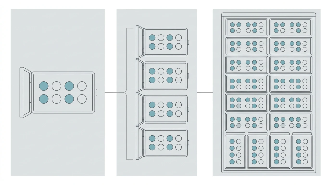
Three habits make that arithmetic survive contact with reality.
- Many outside-plant cables are specified in 12-fiber elements, so the 44 FAT positions required for the year-3 active phase may be rounded to 48 distribution fibers. A full-build design for all homes passed may require additional FAT positions and distribution capacity. The actual cable construction and available cabinet port increments must be confirmed from the selected product range.
- State the spare policy explicitly. Ten percent spare ports on the FAT side and one spare OLT port is a defensible default; zero spare is a decision that shows up as a mid-build redesign. Spare fiber and duct capacity often deserve more attention than spare active ports because later civil expansion may be expensive. The required reserve should be defined by the project’s growth forecast, construction phases and operator policy.
- Watch the two ratios against each other. For the 384-drop example, moving from 1:4/1:8 to 1:2/1:16 halves the FAT count from 48 to 24 and doubles the drops per box from 8 to 16: you buy and install half as many enclosures, but each is larger and puts twice as many homes behind one door. Moving the other way, to 1:8/1:4, doubles the FAT count to 96 for four drops per box. Neither is wrong; pick deliberately, write down why, and re-derive the box count from the level-1 ratio before you commit.
Enclosure ratings, port counts and the cost trade-off
Both boxes are passive, so the specification argument is about mechanical and environmental protection rather than electronics. Select the enclosure IP rating according to the local environment, installation method and the manufacturer’s test conditions under IEC 60529. IP54, IP65 and IP66 may suit different sheltered or exposed locations; IP68 indicates manufacturer-defined immersion conditions and should not be treated as a universal requirement or as a substitute for site drainage and installation design.
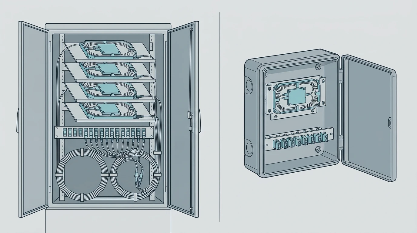
The trade-off that decides most projects is not the rating but the node count:
Factor | Fewer, larger FDTs | More, smaller FDTs |
|---|---|---|
Feeder capacity per site | Higher fiber count per FDT and fewer FDT sites | Lower fiber count per FDT and more FDT sites |
Distribution reach | Longer average distribution runs may be required | Shorter distribution runs may be possible |
Total FAT count | Mainly determined by split ratio, homes passed and service-area geometry | Mainly determined by split ratio, homes passed and service-area geometry |
Distribution-fiber total | Determined by the level-1 ratio and total FAT positions, not by FDT count alone | Determined by the level-1 ratio and total FAT positions, not by FDT count alone |
Civil cost | Fewer sites, but potentially larger foundations and cabinets | More sites, but potentially smaller cabinets and simpler individual sites |
Outage scope | Potentially more subscribers per node | Potentially fewer subscribers per node |
Planned maintenance | Fewer node sites, but larger work areas | More node sites and potentially more site visits |
Two mechanical details deserve a line in the spec sheet because they cause most of the real-world rework. First, bend radius: Where the cable routing or enclosure requires tighter bends, specify a cable construction and fiber type whose installation and long-term bend-radius limits fit the enclosure. G.657.A1/A2 fibers are common choices for tight FTTH routing. The nominal bend-radius values commonly associated with these fiber categories are 10 mm for G.657.A1 and 7.5 mm for G.657.A2, but the final installation and long-term bend-radius limits must come from the selected cable construction and manufacturer’s specification. A cabinet that stores large slack coils must provide enough space to maintain the applicable cable bend radius. Second, adapter orientation: Adapter orientation and internal routing should keep patch cords within their specified bend radius and prevent sharp kinks. Back-reflection is controlled by the specified connector polish and mating interface, not by the angle of the adapter plate, which matters more in a box that a technician opens at night than in a catalog photo.
Installation and serviceability
A FAT that requires unsafe ladder work or exposes technicians to uncontrolled live-roadway hazards indicates a design or access-planning problem, not merely an installation problem. The practical rules that separate a good build from a cheap one:
- Working height. Set the mounting height and working clearance according to local accessibility, worker-safety, road and sidewalk requirements, pole-loading limits, and the operator’s maintenance rules. Values such as 1.2–1.8 m mounting height and approximately 1–1.2 m working clearance may be used as preliminary planning references, not universal installation requirements. Below that, kneeling in wet ground; above that, a ladder for every connection.
- Clearance. Confirm the required working clearance against sidewalk width, road-access rules, local safety requirements and the cabinet manufacturer’s service requirements rather than relying only on the drawing.
- Slack storage. Drops need a service loop; a box with no slack chamber forces splices into the cable tail and shortens the next repair.
- Access route. Pole-mounted boxes need a safe climbing position; wall-mounted boxes need a wall that will still be there in ten years.
- Records. Label the FDT port, the splitter output and the FAT port in one scheme. Fault-finding starts at the splice closure and ends at the right port only if the records agree with the plant.
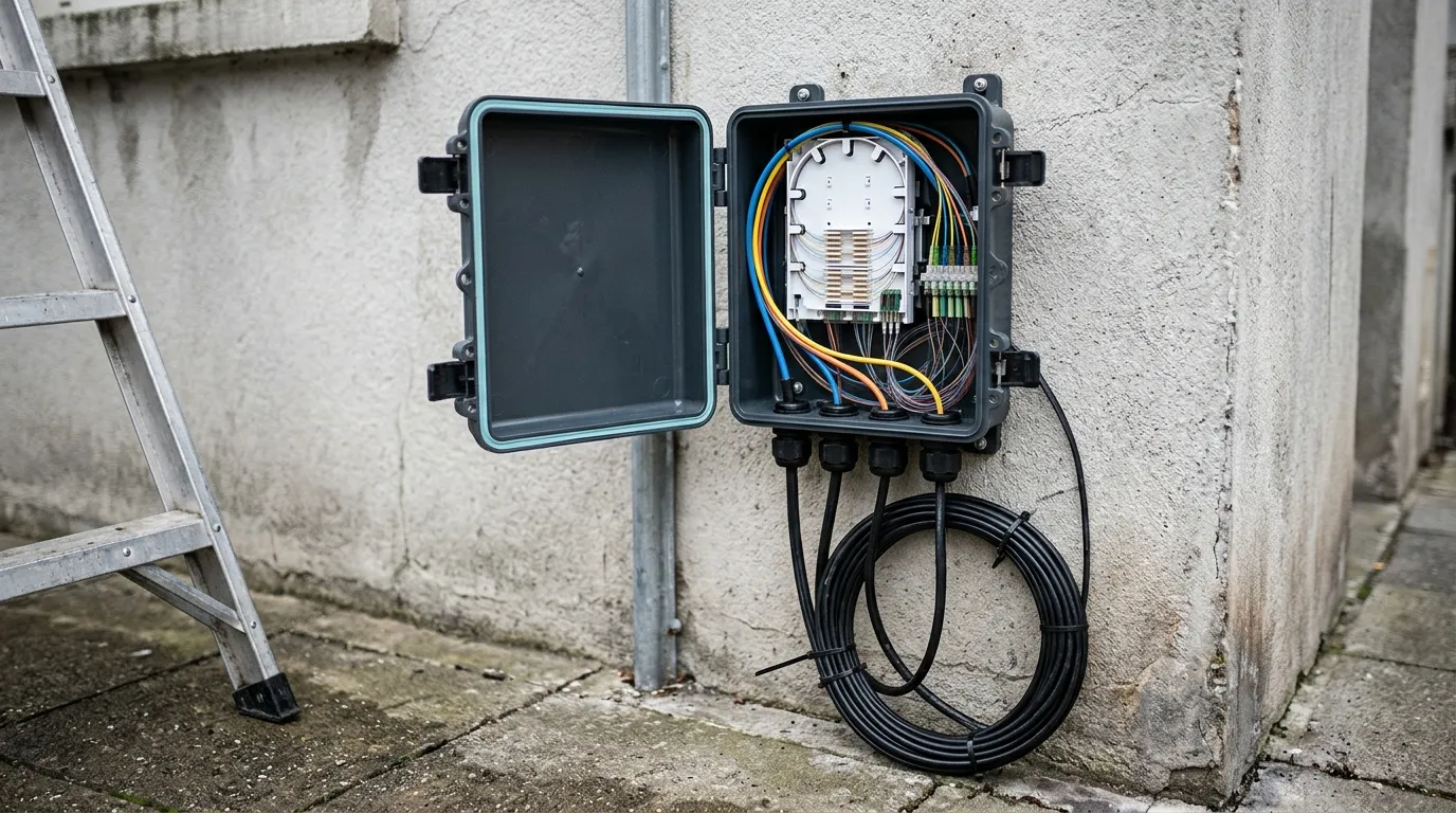
Grounding is the detail people forget. Bond and earth metallic enclosures, messenger wires and associated aerial hardware according to the applicable electrical and telecommunications codes and the project grounding design. Do not assume that the messenger strand is an acceptable grounding conductor. In coastal or high-lightning environments, choose metallic or non-metallic enclosures based on corrosion, mechanical, bonding and lightning-protection requirements rather than material alone. Condensation is the other quiet failure: a sealed box that heats and cools daily will pull moisture through any gland that is not properly sized, which is why vented or breathable designs exist for humid climates.
A decision checklist
Before the order goes out, each line should have an answer on paper:
- Which boundary does this node own? Feeder/distribution → FDT. Distribution/drop → FAT. If a single node is being asked to do both, split it.
- What total split, and how is it divided? Set the target split ratio within the supported optical class and project power budget; 1:32 for GPON and up to 1:128 for some XG-PON/XGS-PON deployments are examples, not universal defaults, then choose the level-1/level-2 pair, then check the optical budget with real splice and connector counts.
- How many homes behind one door? Separate physical coverage from active capacity: use homes passed, drop topology and service-area geometry to size FAT locations and distribution plant; use take rate to size initial OLT ports, installed splitters and staged activation.
- What comes in and what goes out? Feeder and distribution counts set the required capacity; round cable fibers and cabinet ports to the available cable construction and product configuration increments.
- What is the spare policy? Ports, fibers and OLT ports each need a stated number.
- What does the environment demand? IP rating, UV stability, metallic or non-metallic, pole or wall or plinth.
- Can it be serviced safely? Working height, clearance, slack, access, labeling.
- Does the record scheme match the plant? One naming convention from OLT port to subscriber.
FAQ
Is an FDT the same as an FDH? They are often used interchangeably, but the exact meaning depends on the operator’s and vendor’s terminology. "Fiber distribution hub" is the term common in North America, "fiber distribution terminal" in ITU-influenced markets and Europe; both often describe a node where feeder fibers are organized, cross-connected, spliced or split before distribution fibers continue into the access network. Where a vendor distinguishes them, the FDH usually implies cross-connect patching rather than splicing, and often a larger port count.
Can a FAT contain a splitter? Yes, and in distributed-split designs it usually does. A FAT with an integrated 1:8 splitter and eight drop ports is a common second-level implementation in a 1:4 + 1:8 design. A FAT can even carry the whole split in a single-level design, but in that case the node is functionally combining FDT and FAT roles. The feeder/distribution boundary has moved to the remote splitter location, and the upstream cable must be engineered according to its feeder-side optical, fiber-count and loss requirements, even if the operator or vendor continues to call it a distribution cable.
How many subscribers can one FAT serve? Four, eight or sixteen, with eight the most common compromise between enclosure size and node count. The number that matters depends on what is being sized: an 8-port FAT has eight physical drop positions, while at a 55% take rate those eight active connections would correspond to roughly 14–15 homes passed on average. Actual FAT placement and coverage must still follow the address layout and drop topology.
In a conventional passive ODN, the FDT and FAT do not require power; the OLT and ONT/ONU are the powered endpoints. Active remote cabinets, monitoring devices or auxiliary equipment are separate design cases and must be assessed independently. That is precisely why splitter placement, not electronics, is the design lever.
Can you skip the FAT and run drops straight from the FDT? In low-density rural builds where drops are short and few, sometimes. In many suburban grids, it can move the distribution/drop boundary into the cabinet, making each new connection more likely to require a cabinet visit and creating longer drop home runs. The cost shows up later, in operating expense rather than capital.
The short version
The FDT is the last point where you think in cables; the FAT is the first point where you think in customers. Choose the split ratio in pairs, size active capacity from take rate and spare policy, and size FAT locations and distribution plant from homes passed, drop topology and service-area geometry rather than from the datasheet maximum.