FTTH Network Topology Design: How to Plan

FTTH network topology design is the decision that fixes the physical shape of a last-mile fibre network before a single trench is priced. Either every subscriber gets a dedicated fibre back to the head end, or one feeder fibre is shared through passive splitters placed somewhere between the central office and the homes. That single choice decides where your splitters live, how much fibre you buy, whether the optical budget can close, and what it costs to add the next hundred subscribers. This guide treats the subject as one ordered procedure — density and take rate first, topology second, splitter placement third, the optical budget last — which is the part most reference pages leave out. It belongs with the wider FTTH & PON deployment guides for last-mile access.

What "FTTH Network Topology Design" Actually Means

Three words get used as if they were one, and the muddle is where weak designs begin.

• Topology is the physical shape of the fibre route: point-to-point, star, bus, ring, mesh. It describes what the cable physically does.
• Architecture is the technology class: a passive optical network (PON), where the only powered devices are the OLT in the central office and the ONT at the subscriber, or an active point-to-point network with powered switches in the field.
• Splitter placement is the recipe: where the passive splitter sits on the route — in the central office, at a single point in the field, or cascaded across several points.

Design moves through all three in that order. Topology is a network property you choose; architecture is a technology decision you inherit from the PON standard; splitter placement is the engineering response to the first two. The ITU-T recommendations that define PON — G.984 for GPON and G.987 for XG-PON — specify the optical interface and the protocol, not your physical layout. A PON therefore behaves as a logical star even when the cable route branches like a tree, which is exactly why an "architecture" diagram and a "topology" diagram of the same network look different.

It is also worth separating FTTH from its neighbours. FTTC and FTTN stop the fibre at a cabinet or a node and finish the last stretch over copper; FTTH carries the optical path the whole way to the subscriber. That difference is what makes topology a real design question here: once copper is gone from the last mile, the shape of the fibre path is the only thing setting your reach, your loss and your cost.

The Physical Topologies You Can Choose From

Textbooks list a familiar set of physical topologies. Only some of them make sense for access fibre, and the ones that do behave very differently once splitters enter the picture.

The practical reading of that table: residential access is almost always a star or a distributed star, and the design question is not "which shape" but "how many stars, nested how deep." Point-to-point stays in the conversation for business districts and backhaul, where dedicated bandwidth and clean fault isolation are worth the fibre. Ring and mesh earn their place one layer up, in the feeder and metro network that feeds the access star — they are the wrong answer for the drop itself, because the cost of doubling every drop path dwarfs the outage it prevents.

A second consequence is easy to miss: topology sets how many places you must be able to change a connection. A home-run build concentrates every change at the head end, where a patch is minutes of work; a distributed star scatters change points across the field, where each one is a truck roll. Neither is better in the abstract, but the operating model you can actually staff is a real constraint, and it belongs in the topology decision rather than in an operations review two years later.

The choice between point-to-point and a shared star is also the choice between two technology families. An active point-to-point build runs Ethernet to each subscriber; a shared star runs a PON. The trade-offs — dedicated versus shared bandwidth, powered versus unpowered field equipment, port cost versus fibre cost — are set out in AON vs PON network architecture, and they should be decided before you draw any splitter.

Where the Splitters Live: Home Run, Centralized and Distributed Split

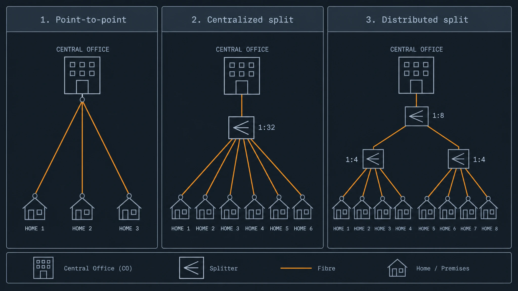
Once you have committed to a shared star, the topology question becomes a placement question. There are three working recipes, and they differ in exactly one thing: how far the splitter sits from the subscriber. They are the classic FTTH architectures, and the FOA's FTTH architecture reference draws the same three-way distinction.

Home run is the most flexible and the most fibre-hungry. Because every subscriber has a dedicated fibre to the head end, the splitter can be fully populated and each OLT port can serve any address in the service area; adding a customer is a patch, not a construction job. It is the natural choice when you expect to lease fibre or host more than one service provider.

Centralized split puts one splitter — commonly 1:32 — in a single field cabinet or hub, with a feeder fibre in and drop fibres out. It keeps every change in one place, which lowers truck rolls, and it is the most common suburban default.

Distributed split cascades smaller splitters, for example a 1:8 near the head end feeding 1:4 units deeper in the field to reach the same 1:32 total. It saves distribution fibre and follows scattered clusters, at the cost of more nodes to power nothing but still document.

All three are built from the same passive hardware, and the splitter itself is the component that defines the recipe. The full menu — planar lightwave circuit versus fused biconic taper, balanced versus unbalanced — is covered in types of optical fiber splitters. What matters for topology is arithmetic: whatever route you take, the split ratios multiply, and the total has to stay inside the PON's design window.

How to Choose: Density, Take Rate and Distance

Here is the procedure the vendor guides skip.

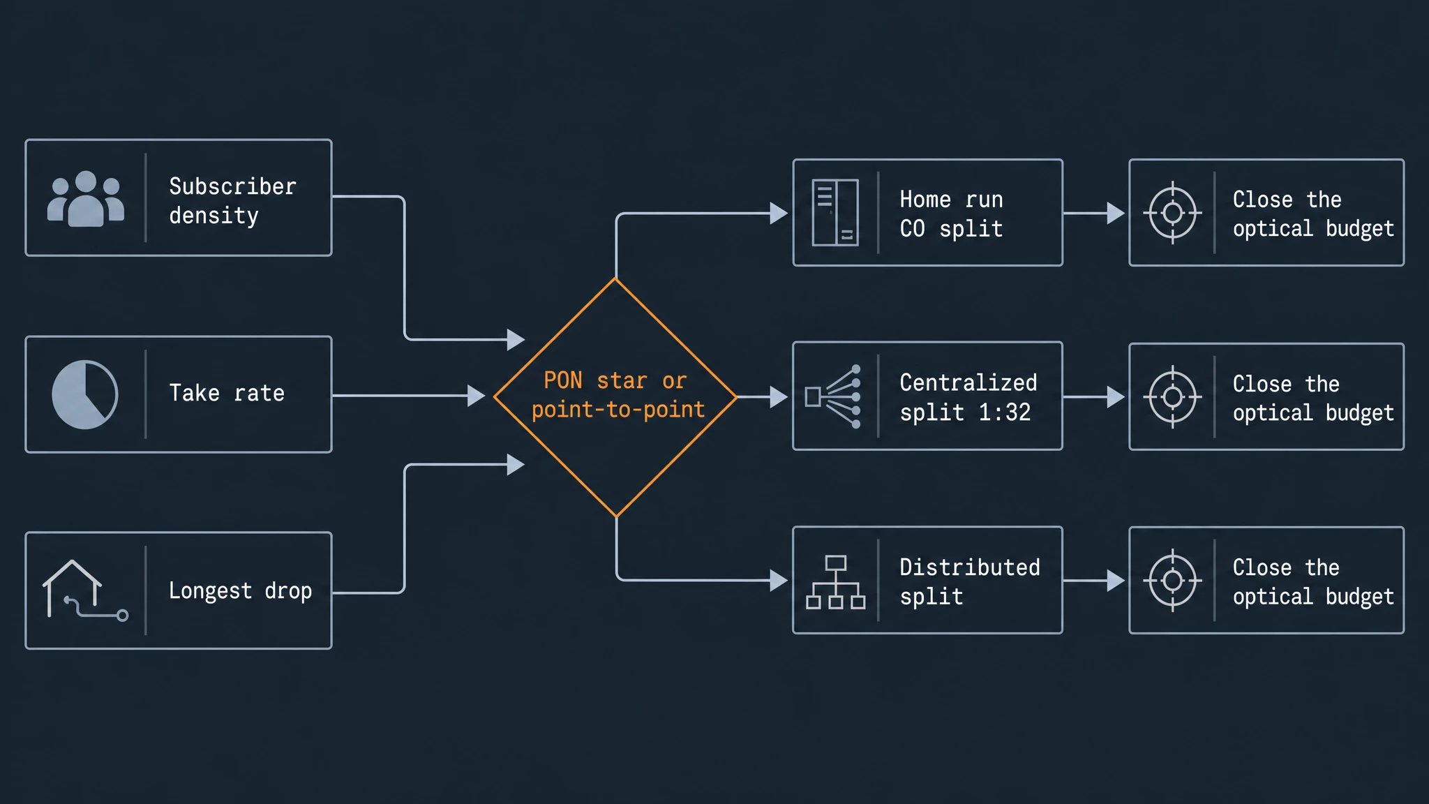
1. Map subscriber density across the service area. Count homes (or units) per street, per block and per building. Density decides how many subscribers one splitter can reach without long drops, and it is the input that changes fastest as you move from a city centre to a rural road. The FOA's FTTH network design reference approaches the same problem by geography — urban, suburban, multi-dwelling and rural — precisely because density drives every downstream choice.
2. Estimate the take rate honestly. Not every home passed will subscribe — common planning practice leaves spare ports for future subscribers rather than assuming 100%. A high take rate favours home run or a fully populated centralized split; a low, uncertain take rate favours distributed splits you can grow into.
3. Measure the longest drop. The distance from the furthest subscriber to the planned splitter decides whether a low-ratio or a high-ratio split is even reachable, and long rural spans may push you toward remote line terminals rather than one distant head end.
4. Choose the topology. High density and high take rate → home run or centralized split. Moderate density → centralized split. Low density and scattered clusters → distributed split, or point-to-point for business.
5. Fix the split ratio and placement. Write down the ratio per splitter and where each one physically sits. This is the output that the cable-plant and budget steps both consume.
6. Close the optical budget. Only now can you confirm the design survives contact with real loss — the step most teams skip until the first link fails to come up.

Two design instincts are worth unlearning here. The first is copying a neighbour's network: density and take rate are local, and a 1:32 build that works in a suburb will strand rural subscribers beyond reach. The second is choosing the split ratio first because the splitter is the part you buy. The splitter is cheap and easy to change on paper; the civil works are neither. Topology first, ratio second.

Making the Optical Budget Close

Every splitter takes light away, and the accumulation is what makes topology a physics problem rather than a drawing exercise. The optical budget — also called the loss or power budget — must be calculated in both directions: downstream (minimum OLT launch power minus ONT receiver sensitivity at 1490 nm/1577 nm) and upstream (minimum ONT launch power minus OLT receiver sensitivity at 1310 nm/1270 nm). The total ODN insertion loss to the furthest subscriber must not exceed the tighter of these two budgets, with safety margin left over. Because single-mode fibre attenuation is significantly higher at 1310 nm (~0.35 dB/km) than at 1490 nm (~0.25 dB/km), the upstream path often dictates the maximum allowable reach.

The contributions are a short list:

• Splitter loss. Each halving of the power costs about 3 dB before excess loss is counted. In round numbers, 1:2, 1:4, 1:8, 1:16, 1:32 and 1:64 splitters cost roughly 3.5, 7, 10.5, 14, 17.5 and 21 dB. The measured figures for real devices are detailed in how much loss a passive splitter adds.
• Fibre attenuation. Single-mode fibre in the access network typically loses around 0.35 dB per kilometre at 1310 nm and 0.2–0.25 dB per kilometre at 1490 and 1550 nm. The cable itself is characterised in the ITU-T G.652 recommendation, with the bend-insensitive variant covered by G.657.
• Splices and connectors. A fusion splice costs on the order of 0.1 dB and a mated connector pair a few tenths of a decibel — small individually, decisive in aggregate across a long cascade.

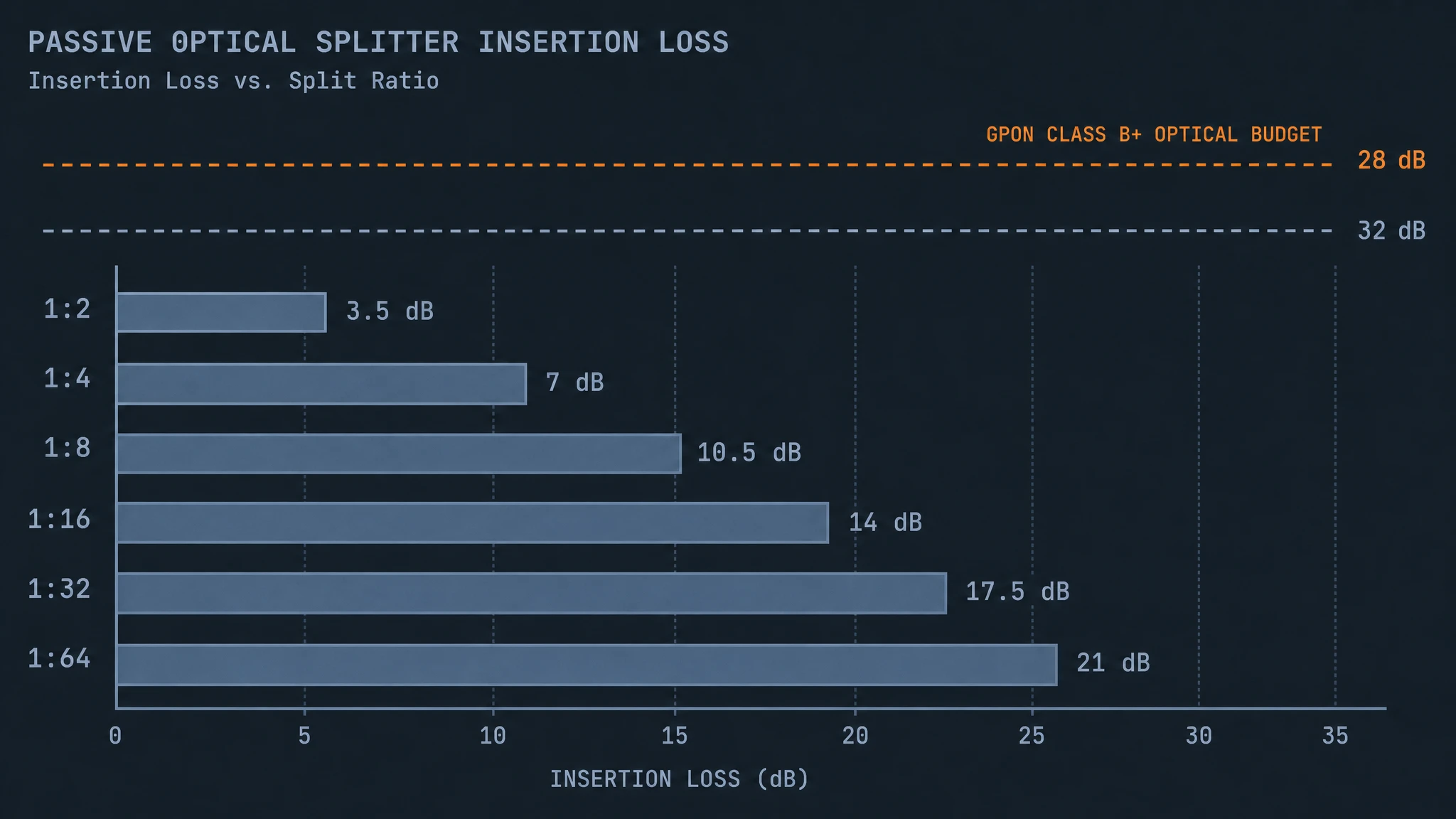
PON standards define the window you are aiming at. GPON is specified with ODN classes — class B+ allows roughly 28 dB and class C+ roughly 32 dB — which is why a high split ratio and a long reach fight each other: choose 1:64 and you have spent most of the budget before the fibre is laid. This is the practical reason topology, split ratio and transceiver class are specified together rather than in sequence. A splitter choice that looks free on a bill of materials can quietly push the network past the point where the link closes.

Design rule of thumb: if the calculated loss to the furthest subscriber lands within a couple of decibels of the limit for the class you are specifying, change the design now — drop a split ratio or shorten the reach — rather than after the first link fails to come up.

Margin is the part of the budget that nobody logs and everybody needs. It absorbs the extra splice someone adds during construction, the connector that gets re-mated, and the gradual ageing that no single technician will notice. A design that closes with 0.5 dB to spare is not passing; it is a network that will throw intermittent faults from the day it is handed over. Budget the reach and the split ratio so that the worst-case subscriber still has a sensible cushion, and the topology survives contact with the field.

Turning the Topology Into a Cable Plant

A topology becomes real as three cable segments, and naming them makes the design reviewable.

• Feeder — the high-count cable from the central office or head end to the first splitter or distribution hub.
• Distribution — from that splitter out to the access points in the streets or building risers.
• Drop — the final span from the access point to the individual ONT.

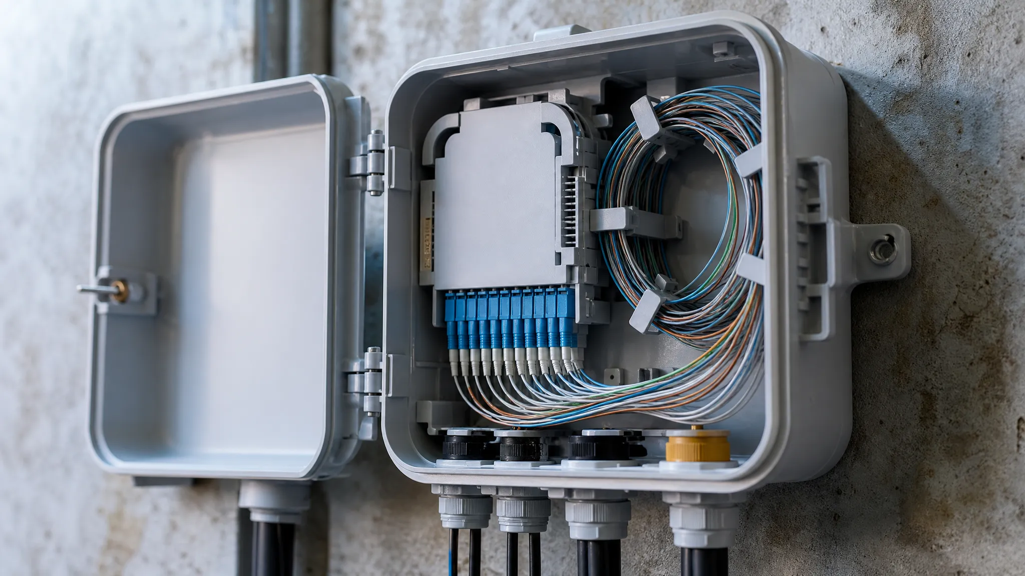
Two hardware families sit along that path. At the splitter node you find the splitter itself, often mounted in a fibre distribution box or a fibre distribution hub; along the distribution and drop segments you find splice closures, terminals and the drop cable. Each is chosen for its environment and its port count, not for the topology, which is a useful separation: the topology is fixed once, the hardware is renewed many times.

Two design documents come out of this stage and repay their cost. The first is a splice schedule — what joins what, at which tray and which port — because an undocumented network lives in one engineer's head until they leave. The second is a bill of materials that traces every component back to a segment and a topology decision, so a costing review can see which choice is expensive instead of just that the total is high. Both are cheap to produce while the design is still a drawing and painful to reconstruct on site.

When the split ratio is set, the splitter is the one component that most directly encodes it. Library-grade planar lightwave circuit modules in the common ratios are the ordinary building block here — as an example of the part, see PLC optical splitters built for exactly these distribution nodes.

Environment, Buildings and the Upgrade Path

The same topology is built two different ways, and the environment can override a preference. Aerial construction is usually faster and cheaper and suits rural and suburban routes where poles already exist; underground is more protected and tidier but slower and costlier, and it dominates congested city centres. Most real networks use both — fibre underground on main routes, aerial on the stretches to individual homes.

Building type changes the last segment. Single-family homes get a straightforward drop from a nearby access point, while apartment buildings are served as a fibre-to-the-building design, with fibre running to a central point and then distributing to units. That distinction is the difference behind the frequently asked FTTH vs FTTB and related terms.

The good news is the upgrade path, and it is a reason to design the topology carefully the first time. Because GPON and its successors use separate wavelengths and the same passive fibre, a network built for GPON can be upgraded to a 10-gigabit class PON over the same cable plant, changing the electronics at each end rather than rebuilding the outside plant. The comparison of generations and what each one changes is set out in GPON vs EPON vs XGS-PON. The constraint that carries forward is the optical budget: a topology that barely closes on GPON will not thank you when the next generation asks for more loss headroom, so leave margin while the design is still cheap to change.

FTTH Network Topology Design FAQ

How do you design an FTTH network? Start with demand, not equipment. Map subscriber density, estimate take rate, measure the longest drop, then choose a topology and a splitter placement that fit those three facts. Only then select split ratios and confirm the optical budget closes. The order matters because each step constrains the next.

What is FTTH network architecture? Architecture is the technology class of the access network — most often a passive optical network, in which an OLT at the head end serves many subscribers through unpowered splitters and an ONT at each premises. It is related to but distinct from topology, which describes the physical shape of the fibre route.

What is network topology design? It is the process of choosing and documenting the physical arrangement of a network — point-to-point, star, ring, mesh and their variations — so that routing, redundancy, reach and cost are decided deliberately rather than inherited by accident. In FTTH the choice concentrates on the shape of the access star and where its splitters sit.

What is the difference between FTTH and FTTP? They describe the same optical path and differ mainly in scope. FTTP is the umbrella term for any fibre-to-the-premises build; FTTH specifically means fibre reaching an individual home. The wider family, including FTTB, FTTC and FTTN, is compared term by term in the FTTH and FTTP definitions article.

Get the topology right and every later decision gets easier: the splitter placement follows from it, the budget can be tested against it, and the cable plant and bill of materials fall out of the same drawing. For the hardware that implements the access layer — splitters, distribution boxes, drop cable and closures — start from FTTH / FTTx solutions.