PON Splitter Ratio Selection: 1:8 to 1:64

The Short Answer: Pick the Splitter Ratio Your Worst Path Can Afford

A splitter ratio is not a preference and it is not a catalogue tier. It is the number of ports whose worst-case insertion loss still fits inside the optical budget you have left, after fibre, splices and connectors have taken their share, with something held back for the day the plant needs a repair.

So the procedure runs in one direction only:

1. Take the loss budget of your PON class.
2. Subtract worst-case fibre loss, splice loss, connector loss and splitter max insertion loss on the worst path in the ODN, not the average one.
3. Keep a design margin — 3 dB is the figure most planning teams work to.
4. Choose the largest ratio that still clears.

If 1:32 clears on your route and 1:64 does not, then 1:32 is the answer even when 1:64 is cheaper per port. Run the same route on 12 km of G.652 fibre with GPON Class B+ optics and the splitter ratio question answers itself: 1:32 lands at about 22.0 dB of the 28 dB available, 1:64 at about 25.6 dB, and only one of those leaves a margin you can live with for fifteen years.

Everything else in this guide — reach, revenue per port, cascade depth, upgrade path — is a consequence of that subtraction. Get the subtraction wrong and no amount of clever topology saves the design.

What a Splitter Ratio Measures, and What It Does Not

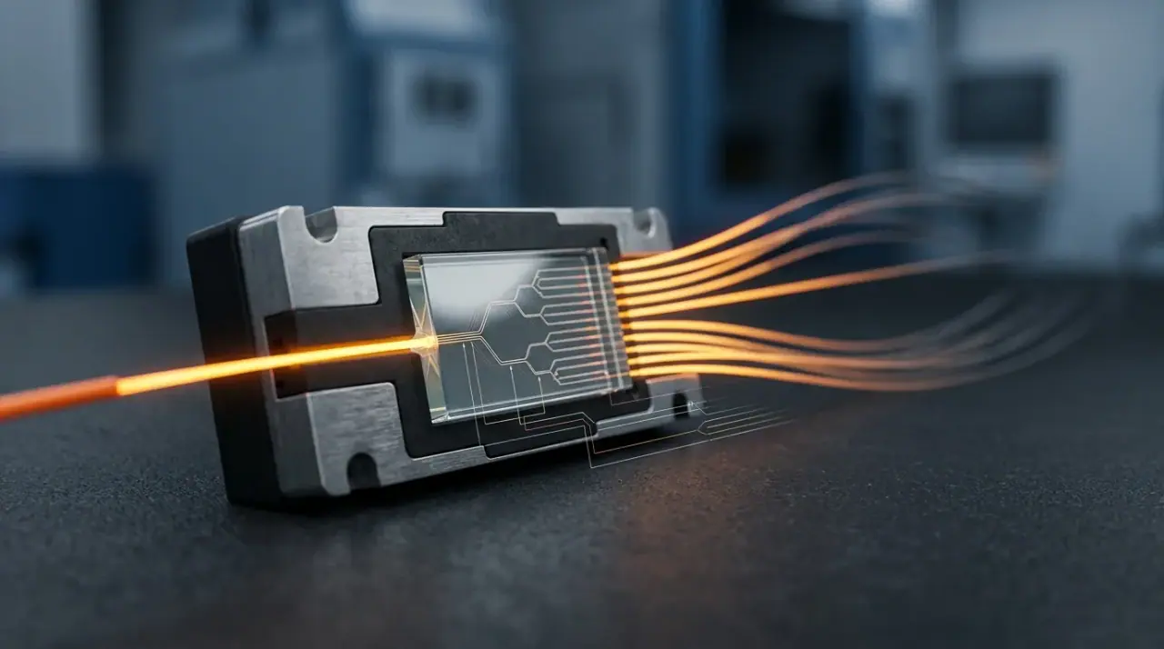
A 1:32 splitter accepts one fibre and delivers the input power across 32 outputs. In a PLC (planar lightwave circuit) device those outputs are balanced: each port gets one thirty-second of the input, minus the device's own excess loss. That is the whole physical story, and it is where most confusion starts.

Three things a ratio is routinely mistaken for:

A subscriber count. It is not. A ratio counts ports. A 1:32 splitter in a 32-home area with 60% take-up serves 19 live subscribers and leaves 13 ports dark. You size for homes passed, you bill for active subscribers, and the gap between them is a commercial assumption you should write down before you order hardware.

A split level. Also not. Ratio is how many ways one device divides the light; split level is how many devices the light passes through. A 1:32 can be built as a single stage (one 1:32 module) or as two stages (1:4 in the cabinet, 1:8 at the access point). Same ratio, different loss, different flexibility. The FTTH and PON deployment guides index covers the topology side of that distinction in more depth.

A loss figure. A ratio tells you the ideal arithmetic, not the guaranteed performance. The number that belongs in your budget is the maximum insertion loss on the datasheet — and the two differ by more at high ratios than most people expect.

One notation note before the numbers, because it wastes real time in tender reviews: 1:32, 1x32 and 1×32 all describe the same part, and a single bid pack will often use all three. Whether a catalogue calls the figure an optical splitter ratio or a fiber splitter ratio, it means the same ratio of input ports to output ports. Compare quotes on the ratio and the loss class, never on the punctuation.

One more distinction worth keeping straight: balanced PLC splitters are the default in FTTH, but FBT splitters can be unbalanced — 90/10, 80/20 — which is what you want for a tap or a legacy video overlay, and what you must not accept when 32 subscribers are meant to receive equal service.

The dB Each Ratio Actually Costs

Ideal split loss follows the port count logarithmically: 10 × log₁₀(N). In practice a commercial PLC module adds excess loss on top, and the excess grows with port count because longer waveguide arrays and tighter alignment tolerances cost more.

Two things follow from that table, and both change designs.

First, every doubling costs about 3 dB, slightly more once excess loss is counted — 3.2 dB per step at 1:32, 3.6 dB at 1:64. Halving your port count buys you roughly 3 dB of margin, which on a long rural route is often the difference between a working PON and a callback.

Second, budget on the maximum, not the typical. Datasheet "typical" values sit 0.3–0.6 dB below the guaranteed maximum. On a single link that looks like rounding; across a fleet it means the ports you actually commission are not the ports you designed for. If the module is specified at 16.9 dB max for 1:32, use 16.9 dB.

The "typical PLC max insertion loss" column is industry-typical rather than anyone's guarantee, so it is worth putting a real datasheet next to it. Our own GPON modules are specified at ≤10.2 dB for 1x8, ≤13.5 dB for 1x16, ≤16.5 dB for 1x32 and ≤20.5 dB for 1x64 — 0.2 to 0.4 dB tighter than that column up to 1x32, and level at 1x64. If your quote states no maximum, budget the industry-typical figure shown here and put the maximum on the PO before you order.

The same table settles quote comparisons. A 1x16 splitter costs 3.2 dB more than a 1x8 splitter, and a 1x32 splitter costs 6.4 dB more than that same 1x8. Put 6.4 dB back into fibre terms at 0.35 dB/km and you get 18 km — more route than many suburban cabinets have to spend.

Insertion loss also drifts with wavelength. PLC modules are usually specified at 1310, 1490 and 1550 nm separately, with the 1310 nm figure marginally worse. Since upstream traffic on GPON runs at 1310 nm and XGS-PON upstream at 1270 nm, the upstream direction usually sets the worst case on a long route. PON splitter loss is therefore a two-part number — the ideal logarithm plus the device's excess — and only the second part belongs to the vendor you choose. The splitter loss breakdown for each ratio goes deeper into where those numbers come from and how they are measured.

Reading the Ratio Off a Real PON Budget

Numbers are easier to trust when you can see them subtracted. Take a suburban route: 12 km of G.652.D single-mode fibre from the OLT to the furthest ONT, three fusion splices, one connector pair at the OLT patch panel and one at the customer, and a single splitter. GPON Class B+ optics.

A link budget is only as good as its worst line, so build it line by line rather than from a remembered total. The receiving end matters too: ONU sensitivity is quoted in dBm, and the budget class already folds transmit power and sensitivity into one number, which is why the class matters more than either endpoint on its own.

Change one line of that table and the answer moves. A 1:64 splitter at 20.5 dB pushes the total to 25.6 dB and leaves 2.4 dB — under the 3 dB reserve, which means the first repaired cable section or the first extra splice eats your design. A 1:16 at 13.7 dB leaves 9.2 dB, comfortable, but you have just spent one OLT PON port on 16 homes and will need a second port a year earlier than necessary.

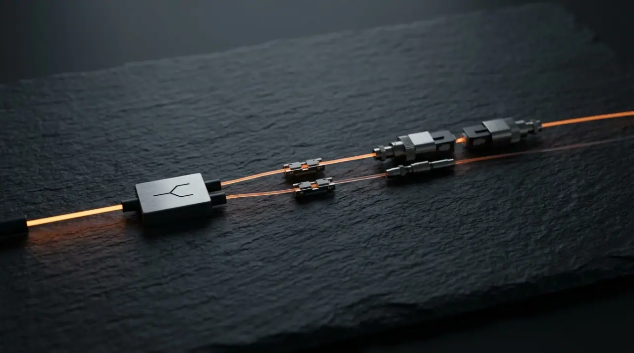
That 3 dB reserve is a working rule, not a clause in a standard. It covers repair splices after a cable cut, temperature-driven loss change, the difference between as-built and as-designed lengths, measurement uncertainty on the power meter, and one future mid-span tap. Some operators hold 2 dB on short urban routes and 5 dB on aerial plant. Whichever figure you adopt, state it in the design document so the next engineer knows what the margin was for; the acceptable dB loss discussion covers how those reserves are typically set.

The optics class is part of the same decision

Here is the part most ratio guides skip. A 1:64 splitter that fails on Class B+ passes comfortably on Class C+, because the budget moves from 28 dB to 32 dB and the margin at 25.6 dB goes from 2.4 dB to 6.4 dB. Choosing a higher-budget optics class is often cheaper than choosing a lower split ratio, since it buys PON port capacity without buying more fibre or more OLT cards.

The same logic runs across generations. XGS-PON defines its own attenuation classes — N1, N2 and E1 at roughly 29, 31 and 33 dB — so a ratio that is marginal on GPON may be routine on XGS-PON optics over the same glass. The optical budget classes are set in the PMD layer of each standard: ITU-T G.984.2 for GPON, G.987.2 for XG-PON and G.9807.1 for XGS-PON. Read the current edition for the exact class figures you are procuring against; they are the numbers your link must satisfy.

If you would rather compute per route than read a table, our optical splitter loss calculator applies the same arithmetic to a full path including fibre, splices and connectors.

Ratio, Reach, and Where a High Split Stops Working

Distance is the second constraint, and it binds at different ratios than people expect. Strip out the splitter and the reserve, and what remains is the dB available for fibre and splices.

On Class B+ at 28 dB, a 1:32 splitter leaves about 8 dB for the route after the 3 dB reserve — roughly 23 km of pure fibre at 0.35 dB/km, so 18–20 km once 1.1–1.8 dB of splice and connector loss is deducted. A 1:64 leaves 4.5 dB, about 13 km of fibre before splices and closer to 10 km built. That is why dense suburban estates with cabinets 3 km from the OLT can run 1:64 while the same equipment at 15 km cannot.

Two numbers govern G.652.D attenuation, and they are routinely confused. The first is what you can buy: Prysmian's G.652.D fibre datasheet, for example, specifies ≤0.35 dB/km at 1310 nm and ≤0.21 dB/km at 1550 nm. The second is what the standard requires, and it is looser: ITU-T G.652 sets a statistical cable limit for G.652.D of 0.40 dB/km anywhere from 1310 nm to 1625 nm, with 0.30 dB/km over 1530–1565 nm. The 0.35 dB/km used throughout this guide is the first of those numbers, so it only holds for cable whose purchase order states it. Buy on price without an attenuation figure and the binding number is the standard's 0.40 dB/km — and every reach figure below shortens accordingly.

The gap between the two wavelength windows is why a downstream-only calculation flatters a long route: at 1490 nm the same 12 km costs about 3.0 dB at a conservative 0.25 dB/km, against 4.2 dB at 1310 nm. Design on the upstream wavelength and the downstream will take care of itself.

One honesty check before you push a ratio to its loss limit: physical reach is also capped by the standard, independent of loss. GPON and XGS-PON are specified for a 20 km physical reach with a 60 km logical reach, so a low ratio on a high-budget class can have plenty of optical margin and still be out of spec on distance. Where loss bites first, the ratio is your lever. Where the standard bites first, it is not.

Rural and long-reach designs resolve this by going the other way: 1:8 or 1:16 on Class C+ optics, accepting fewer homes per port in exchange for reaching them at all. A 1:16 on C+ at 32 dB leaves 15.3 dB for the route — about 43 km of fibre by arithmetic, capped at 20 km by the standard. On a route that long, the constraint is real estate and splice count, not port count.

Sizing by Served Subscribers, Not Port Count

Once the ratio clears the budget, the remaining question is commercial: how much capacity are you selling per port? Two numbers decide it, and only one of them is usually checked.

Downstream. GPON delivers 2.488 Gbps shared across the PON; XGS-PON delivers 9.953 Gbps. Compare that with the sum of the service tiers you sell on the port.

Upstream. GPON carries 1.244 Gbps upstream. At 1:64 with 20 Mbps upstream per subscriber sold, 64 subscribers can theoretically ask for 1.28 Gbps — more than the port has. That is the constraint that shows up first in a market with heavy video calling, cloud backup or symmetric small-business traffic, and it is invisible if you only model downloads.

Read that table as a worst-case bound, because it assumes every port on the PON is sold at that tier. At the 60% take-up used earlier, 1 Gbps service on a 1:64 XGS-PON port is about 38 live subscribers asking for 38 Gbps — roughly 3.8:1 against the 9.953 Gbps port, not 6.4:1.

Those ratios are survivable because subscribers do not all peak at once. Most operators plan for a peak oversubscription somewhere between 4:1 and 8:1 depending on market and contention policy, which puts 1 Gbps service on a sold-out 1:64 XGS-PON port at the edge of comfort and 1 Gbps on a 1:32 in the normal band. If you are weighing GPON against XGS-PON for the same estate, the GPON versus XGS-PON comparison puts the capacity and cost sides next to each other.

The practical rule: a ratio is only "too high" when either the optical budget or the sold capacity fails. A 1:64 that passes the budget on 100 Mbps service is a good design. The same 1:64 selling 1 Gbps on GPON is a support queue with a fibre connector on it.

Cascaded Splits: What 1:4 + 1:8 Really Costs

Cascading is sold as flexibility, and it is — but the flexibility has a price in dB, and the price is rarely quoted.

A 1:4 followed by a 1:8 gives you 1:32 overall. Splitter loss is 7.3 dB plus 10.5 dB, so 17.8 dB, against 16.9 dB for a single 1:32 module. That is 0.9 dB more for the same port count. Add the two extra mated connector pairs that a second stage usually introduces, at 0.3 dB each, and the real penalty is about 1.5 dB.

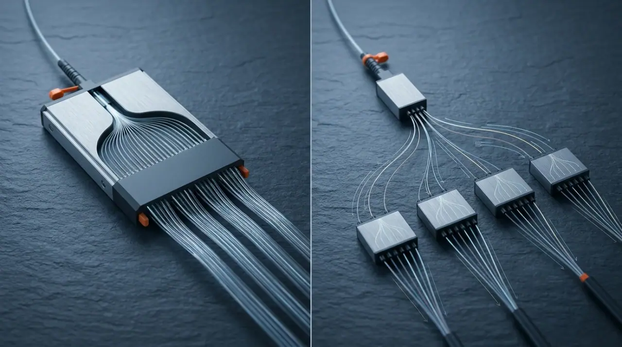
A decibel and a half does not sound like much until you put it back into the reach equation: at 0.35 dB/km it is 4.3 km of fibre. On a 6 km suburban route, cascade and pay it. On an 18 km rural route, it may be the difference between passing and failing.

Cascade still wins in four situations. You save feeder fibre because a single 4-fibre cable reaches a neighbourhood instead of 32 fibres reaching 32 homes. You can build in stages and light up a second cluster from the same feeder later. You shorten the drop cable runs in dense multi-dwelling buildings, where the in-building splitter sits a few floors from the customer. And you gain fault isolation, because a fault on one second-stage leg takes out 8 subscribers rather than 32.

The design discipline is to model the cascade as one path — both stages, both connector pairs, every splice between them — rather than as two independent choices. The FTTH network topology design guide works through the cabinet and access-point split patterns that keep the penalty small.

A Ratio Decision Table, by Deployment

Treat every row as a starting hypothesis, not a rule. The route in front of you decides, and the numbers above only tell you which splitter ratio is worth testing first.

Keeping the Option Open

A splitter ratio is easy to design and expensive to change. Replacing a 1:16 with a 1:32 means a new module, new pigtails, a re-splice, a new as-built record and a maintenance window — usually at the worst possible moment, because demand is what triggered it. Three habits make the change cheap:

Leave ports dark on purpose. A 1:32 splitter with 19 subscribers has 13 spare ports. That is not waste; it is the cheapest capacity you will ever buy, and it is already installed.

Use modular splitter shelves instead of potted modules. A plug-in tray that accepts a 1:16 or a 1:32 card lets you upgrade the ratio without touching the feeder cable or the closure.

Record as-built loss per port. Measure every port at commissioning and file the numbers with the route. Do it with a light source and power meter rather than an OTDR trace: a splitter presents a large step loss and a short dead zone, so a single-ended reflectometry trace will not give you a trustworthy per-port insertion loss. When a subscriber reports slow service two years later, a measured baseline tells you whether the plant degraded or the service tier was always marginal. The FOA's guidance on testing couplers and splitters covers the measurement setup; the discipline of keeping the results is yours.

What to Specify on the Purchase Order

The ratio on the drawing is not the ratio you receive unless the order says so. Six lines turn a design intent into a delivered part:

• Maximum insertion loss per port, stated at 1310, 1490 and 1550 nm — not "typical", and not a single wavelength.
• Uniformity, the maximum spread between the best and worst port. A 1:32 with 3 dB of spread has a worst port that sets your design, whatever the average says.
• Return loss and directivity, typically ≥55 dB for APC-polished ports in FTTH.
• Connector and polish: SC/APC with 8° endface for outside plant, with the pigtail length and tolerance you actually need.
• Test evidence: per-port measured loss with the method stated (IEC 61300-3-4 is the common reference), and qualification to GR-1209/GR-1221 or the equivalent your operator accepts.
• Form factor and footprint: bare-fibre, ABS box, plug-in splitter tray or 19-inch shelf, matching the closure or ODF it will live in. A module that does not fit the tray becomes a field modification.

As a manufacturer we build GPON splitter modules across the 1:4 to 1:64 range, and the specification argument above is the same one we have with buyers every week: the ratio is the easy part, the guaranteed per-port loss is what the network lives with.

Mistakes That Only Surface After Cutover

Most of these mistakes share one root: a splitter ratio chosen from a catalogue page or a colleague's last project, instead of from a subtraction on the route in front of you. Each one below is worth checking against your own design before the cable is pulled.

Designing on typical loss. The design passes on paper and one port in twenty misses at commissioning. Always budget the maximum.

Forgetting the upstream window. Downstream at 1490 nm looks comfortable while upstream at 1310 nm is 1.2 dB worse over 12 km. On long routes that gap decides the ratio.

Sizing to 100% take-up. A port fully consumed by homes passed cannot be sold twice, and churn leaves you with ports you paid for and cannot reallocate.

Cascading without the connector loss. The second stage is not just a splitter; it is a splitter plus the patch cords that reach it. Add both.

Assuming 1:64 is simply cheaper per port. It is cheaper per port and more expensive per repair, because every fault on the feeder now affects 64 subscribers and every margin problem is shared.

Buying a ratio but not a uniformity figure. The worst port, not the average, is the one that generates the trouble ticket.

No as-built baseline. Without measured per-port loss at commissioning, nobody can tell degradation from a design that never had margin.

FAQ

Is 1:32 or 1:64 the better choice for GPON?

1:32 is the safer default for GPON residential plant, because it clears a Class B+ budget with usable margin out to roughly 18–20 km on a lightly spliced route, allowing 1.1–1.8 dB of splice and connector loss on top of the 3 dB repair reserve, and it keeps the upstream from being the binding constraint. Move to 1:64 when the route is short, the optics class is higher, or the service tiers are modest — and only after the worst-path arithmetic clears your reserve.

Can a PON run a 1:128 split?

The standards can address 128 ONUs on a PON, but the optical budget rarely cooperates: 1:128 costs about 21 dB of ideal split loss before excess loss, which leaves almost nothing for fibre on a normal class. Commercial 1:128 deployments exist in very short-reach, high-budget designs; treat it as an exception to be calculated, not a tier to select.

Do cascaded splitters cost more loss than a single splitter of the same ratio?

Yes. Two stages of 1:4 and 1:8 total 17.8 dB against 16.9 dB for one 1:32 module, and the extra connector pairs typically add another 0.6 dB. The cascade buys feeder savings and staged build-out; it does not buy optical performance.

When do I need an unbalanced splitter?

When the branches are not meant to be equal: a tap that monitors a live fibre, a legacy video overlay riding a separate wavelength, or a design where one leg serves a business customer and the rest serve residences. Balanced PLC modules are the right default for subscriber-facing splits, and an unbalanced FBT device is the right answer for asymmetric taps.